Backup-fall simulator

My name is Augustin, I’ve been highlining for almost 10 years. I’m a gear nerd, and I know some programming.

In the past weeks, I developped a highline backup-fall simulator that I made available as a beta version. I’m writing this for highliners that are curious to understand the physical and mathematical ideas behind it. If you do not know what a highline is, it might be a good idea to first check out the ressources on the ISA website , in particular this document, that explains in technical terms what a highline is.

To my knowledge, it is the first backup fall simulator that takes into account the complexity of modern highline rigging. In the last year, I don’t remember a single highline I’ve been on where the main and backup webbing were not connected in some way.

Give back to Ceasar…

A widely known backup fall simulator is the one developped by Panos Athanasiadis available on his website . It takes all the necessary parameters to compute the forces in a backup fall, with a slackliner starting in the middle of the line.

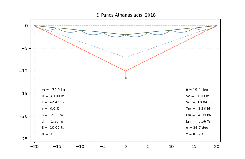
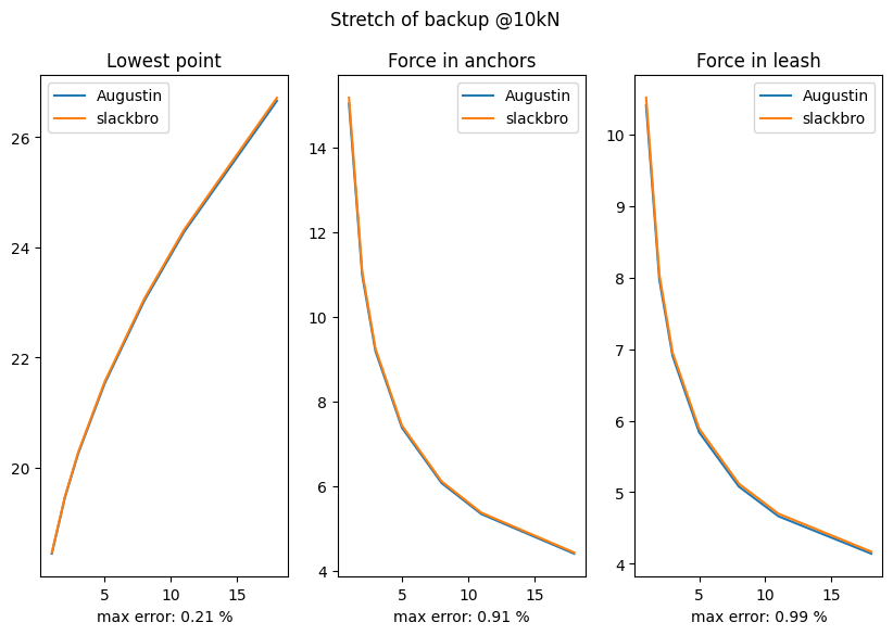
I have used the interface to his model to verify that my model gives similar results in the relevant cases: the highliner is in the middle, and there is no connection between mainline and backup webbing. Since I have less than 1% difference in all the cases I tried, I believe we used the exact same physical model, and that only a few differences in the computational scheme used to solve the equations created the little differences we had. If you’re versed in programming, you can check the full report of this comparison.

I will explain this physical model and the computational scheme, I hope in a way that’s understandable to anyone with a knowledge of highschool science, and with motivation.

Newton’s first law

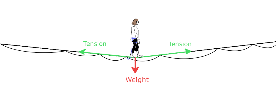
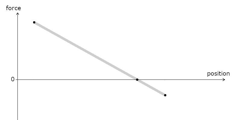
Newton’s first law of motion states that an object doesn’t move if all the forces applied to it balance, i.e. their sum is 0. When a slackliner is on the line, the forces that are applied to them are the weight, coming from the earth’s attraction, and the force that the webbing applies through the feet of the slackliner, that keeps them in the air. This force results from the tension in the webbing, which can in turn be derived from the elongation of the webbing. That’s why we have stretch charts.

Actually, we simplify this by assuming the stretch is directly proportional to the elongation. This is mostly to make it possible for the user to enter the stretch easily through the interface. It would be nice to be able to enter a full stretch curve, and that might be implemented in a future version of the app. For now, the stretch curves we consider will look like this:

Note that we have switched the axis: this makes more sense as we will want to know what the tension is for a given stretch. It will also make more sense when we will run energy computations later.

Now we can know how much tension is in a piece of webbing by knowing its characteristics and measuring its length. Let’s look at the sum of forces again. The weight is vertical, constant. The tension along each piece of webbing gives a force proportional to the extension, directed along the webbing. We represent these forces graphically by vectors (arrows) that point in the direction of the force, and whose length is proportional to the intensity of the force.

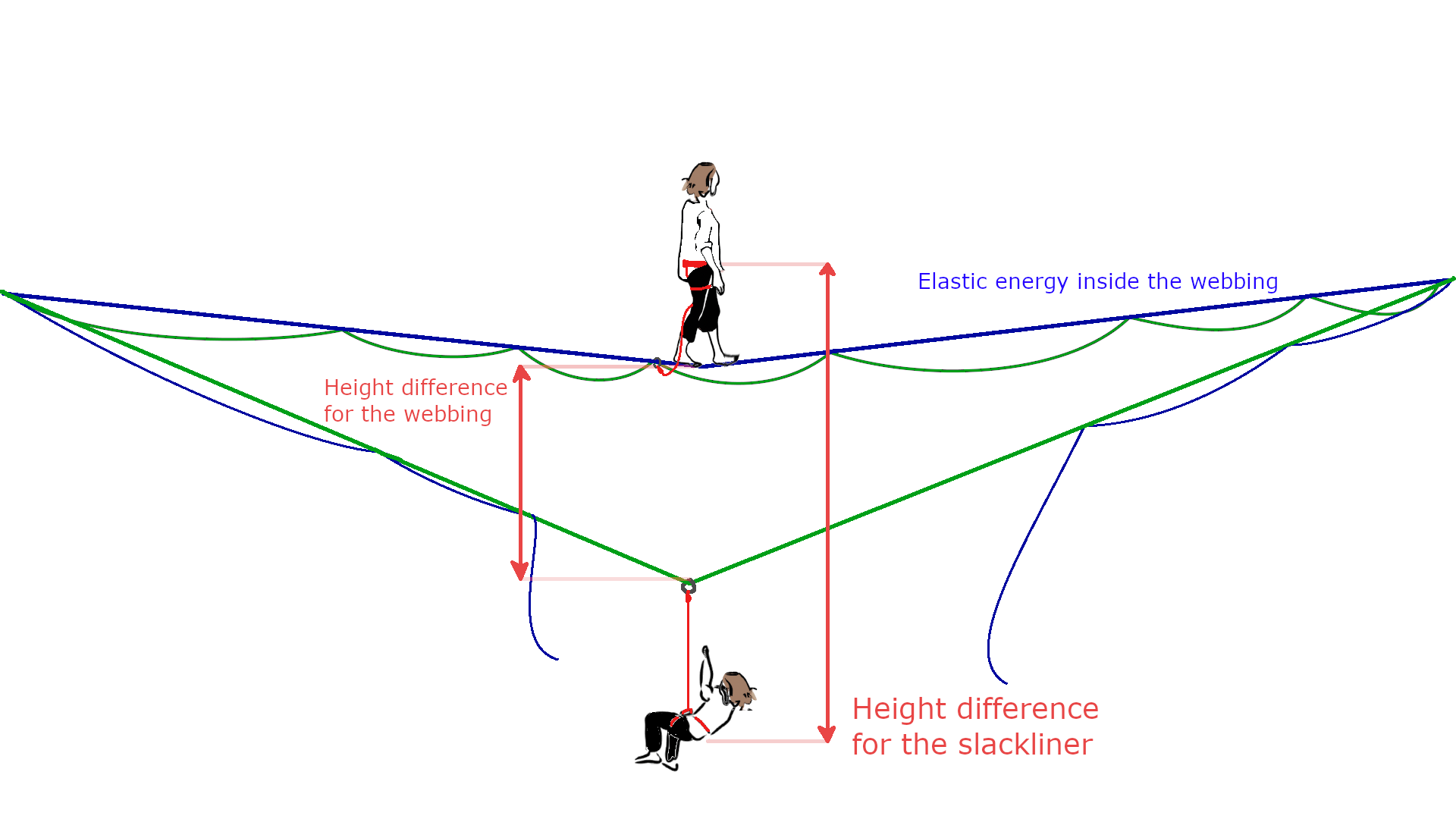
In the simulation, you can decide how far along the webbing the slackliner is, essentially attaching the slackliner to a point on the line. This creates two independent pieces of webbing, one on the left, and one on the right, and when we give some coordinates to the program, it can compute the stretch of each piece of webbing, and the forces resulting.

Each vector force gets split into an horizontal and a vertical component. For the weight, there is no horizontal component. For the tension of the webbings, we project along the horizontal and vertical axis. This way we get the sum of force in the horizontal direction and the sum of forces in the vertical direction.

So, we have this piece of program that you feed a position, and that returns the force in the horizontal direction, and the force in the vertical direction. How do we use that to find the point where the forces balance?

Newton’s method

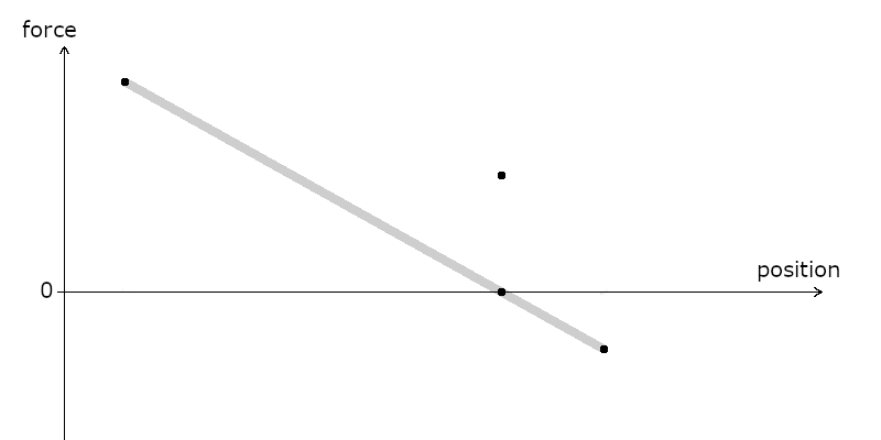
Newton was not only a great physicist, he also had great mathematical ideas. Our goal is to find a point where the sum of the forces cancels out. Newton’s idea was to improve our guessing game by looking at the variations of the function we are studying. The idea is in essence really simple. Imagine you know two values values of a function, and you want to guess where the zero value of that function is.

You might guess that the point you’re looking for is on the line between these two points, like this:

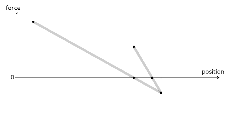
But then, you can run the program again, and it tells you that the actual value of the function at that point was higher:

Well, you just apply the same principle again:

If the actual function you were trying to find the zero off looks like this below, you can understand that this approach is going to get really close to the value you want fast.

💡

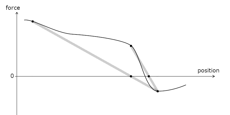
Remember, you don’t actually know this curve, it’s only on this last graph to help understand the process. It would take too much time to compute the value for each point.

Here, we started with one point where the value was positive, and one point where the value was negative. The beauty of this process is that it works even when the values are both positive (or both negative). You just do the same thing, but expand the line outside of the two points to see where it crosses the zero line.

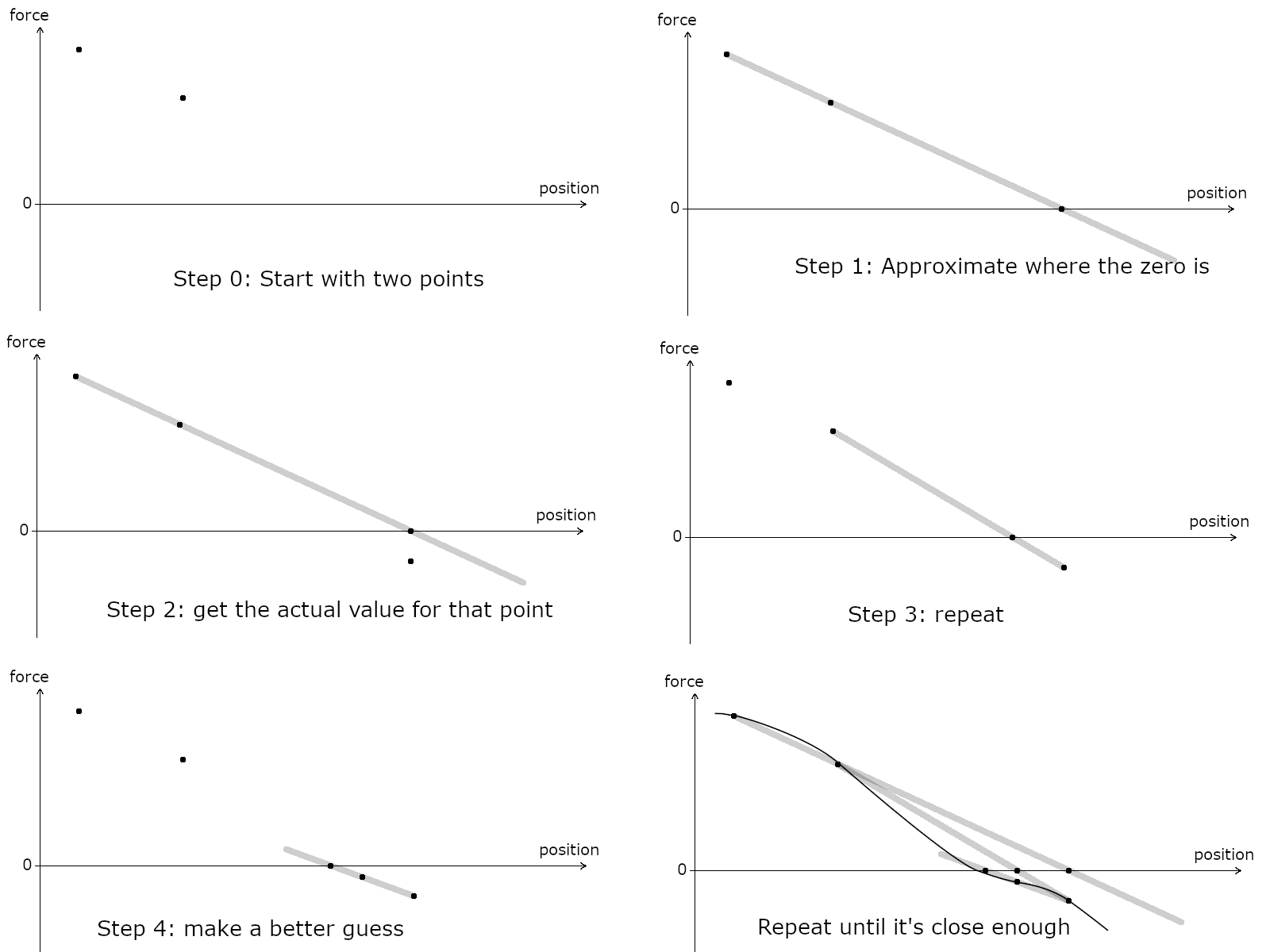
So now we have all the ingredients to find out the sag that the line has with the slackliner on it. We just need to find a good pair of starting points. Here’s the structure of the algorithm:

Algorithm to find the static position of the slackliner:

Starting points: Position of the line with no weight on it, and the same one meter lower;

Do one iteration of Newton’s method in the vertical direction;

Do one iteration of Newton’s method in the horizontal direction;

Repeat as long as the changes in each iteration are more than 1cm;

From the final position, compute the tension in each piece of webbing.

But wait, what happened to having a split set-up?

So far, we have not done much different from the SlackBro model. There is one problem with split setups, that every freestyler is familiar with: tight backup! Indeed, if one section of backup gets tight, the stretch behaviour of the line changes.

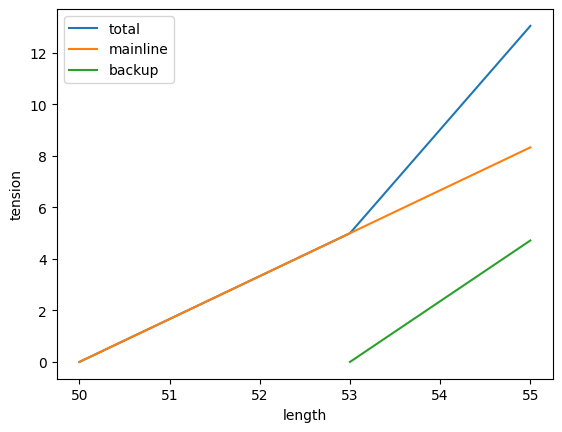
For example, take a mainline webbing that is 50m long, and the back-up of the corresponding section is 53m. What happens is that for the first 3 meters of stretch, you only feel the force of the main line, but after that you also feel the tension from the back up webbing. The two forces add up. Graphically, it looks like this:

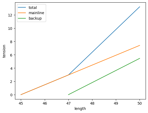
Now, how do we connect two segments end to end? Let’s take another segment, with slightly different characteristics. You can read from the graph below that for this second segment, the mainline is 45m, and the backup is 47m.

Imagine you put the two setups end to end. They start with a length of (50+45) meters, and stretch out as the tension increases. When the tension reaches around 3kN, the backup of the second section gets under tension. We read what the length of the first section is at that tension, and we know the length of the full setup at 3kN. When it reaches 5kN, the backup of the first section also gets under tension. We read the length of the second section at that tension, and we know the length of the full setup at 5kN.

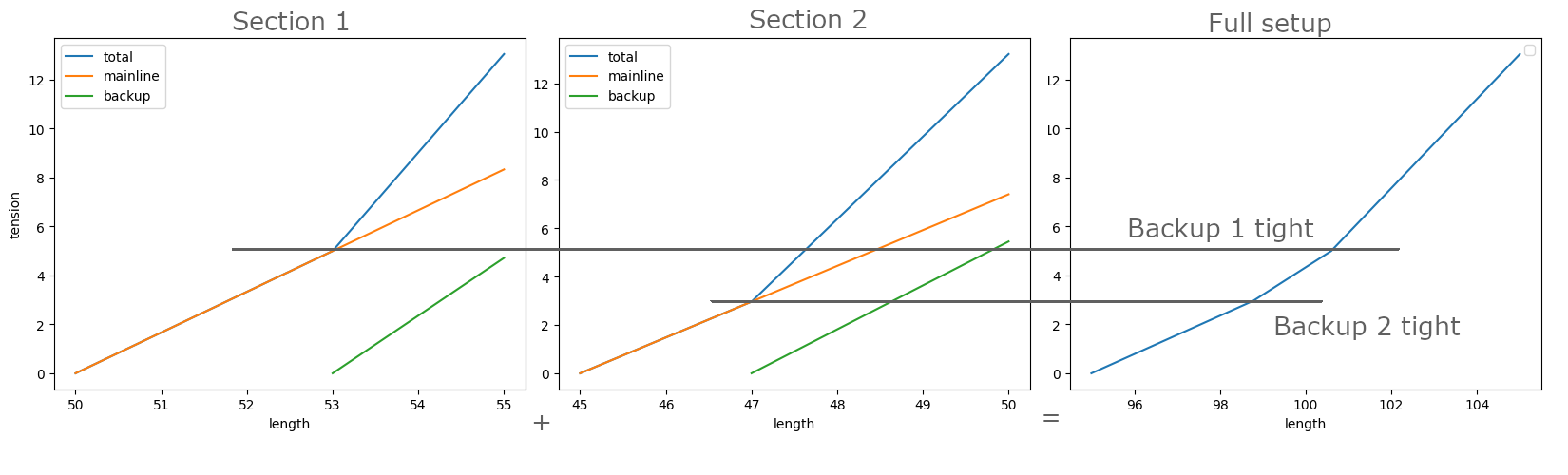
We repeat this for every section of the setup, and get the curves on which we can read what the tension is for any given length. Plug this into the algorithm above, and you can compute the static position of the slackliner.

If we want to compute a backup fall where one segment fails, we will simply need to compute again the stretch curve of the whole system, but we will ignore the mainline for that particular section. The calculations from the next section are the same, whether we are considering a leashfall or a backup fall, only the stretch curve changes.

Let’s do a fall!

Sir Isaac Newton is famous for falls, and yet the principle we are going to use for this computation is not named after him.

What we are using is the conservation of energy. This principle states that in any physical system, there is no energy appearing or disapearing out of nowhere. In this highline modelisation, there are 3 different kinds of energy we will consider:

Kinetic energy, which is the energy associated with moving objects;

Elastic potential energy, which is the energy stored in a spring, or in our case, in webbing;

Gravitational potential energy, which is the energy related to the height of an object.

In an actual highline, there are more kinds of energy. For example, there is chemical energy, stored in your cells, that can be used to make your legs push on that webbing. This creates bounce, which is a cycle of transfer between the three energies above.

At the top of the bounce, you have no speed and the webbing is the least stretched, but you are at the maximum of the gravitational potential energy.

As you go down you pick up speed, kinetic energy increases and gravitational energy decreases, but the webbing is starting to store some energy.

At the bottom of the bounce, all the kinetic energy is gone, gravitational potential energy is at a minimum, it’s all stored inside the webbing, ready to lift you up again.

💡

Bounces don’t last forever unfortunately, that’s because some of that energy gets dissipated, mostly in friction with the air. That’s why you need to keep pushing it.

What interests us for the algorithm is the lowest point of the fall: this way you can know if you will hit the ground. It is also the point where the webbing is the most stretched, and sees the highest tension. The other point we know is the starting point, with the slackliner standing on the line. The good thing is that we don’t have to deal with kinetic energy: in both those positions, the speed is zero.

💡

This is actually a worst case assumption! In most falls, there will be a swinging movement, which means that not all of the kinetic energy is gone. But it’s best to assume the worst.

The area under the curve…

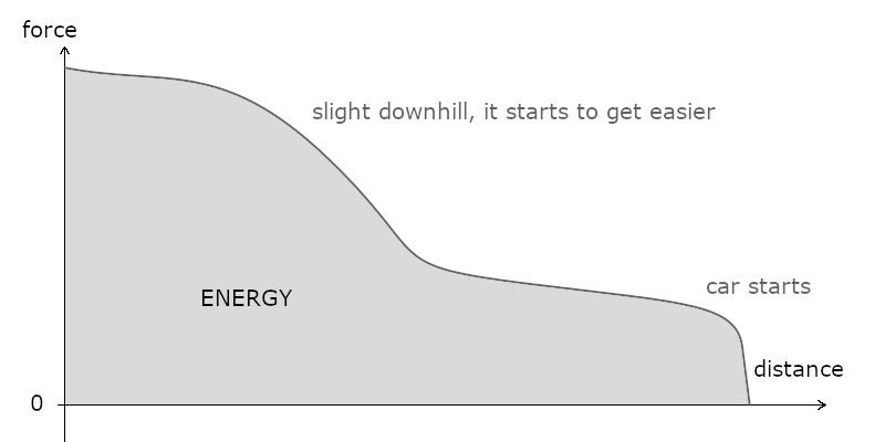
If you’re trying to push a car along a road, the energy you’re putting into that work is equivalent to the force necessary to push it, mutliplied by the distance before the driver who forgot his lights on manages to start the engine. Actually, pushing the car might be harder at the start, easier towards the end. In the end, the energy transferred to the car is proportional to the area in grey on the graph below.

Let’s apply this to the two kinds of energy we are computing.

Gravitational potential energy

Unless you are bouncing into outer space like those BounceKult monkeys, the gravitational force on your body is constant (9.81x weight). This means that the curve is flat. The area under the curve is simply the travel distance (difference of height) multiplied by the gravitational force.

💡

I can choose whatever point as a reference point to compute the energy. What is important is the variation of energy. So for example, in the program, the gravitational potential energy is zero at the point from which the slackliner falls.

The program also takes into account the weight of the webbing. So the webbing has its own gravitational potential energy.

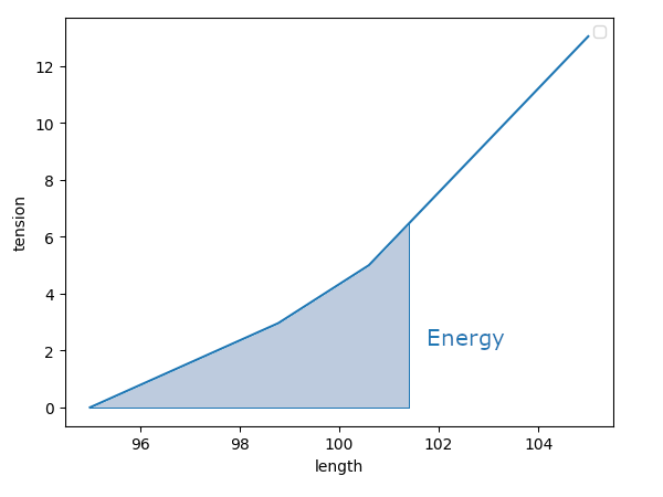
Elastic potential energy

In the stretch curve that we got before, the horizontal axis is the change in length, the vertical axis is the corresponding force. Therefore, the energy stored inside the webbing stretched to a given distance is exactly the area under that curve.

For any position of the highliner hanging in the leash, it is now possible to compute their gravitational potential energy as well as the elastic potential energy stored inside the setup. We put this into a part of the program, that we can reuse anytime we need it.

Now we have all the ingredients to tell the computer how to find the lowest point of the fall. We just need to find the lower point where the sum of the energies is the same as the original sum of energies. Newton’s method can be used in the same way as before, the only difference being that instead of trying to find the point where the sum of the forces is 0, we try to find the point where the sum of the energies is equal to the original energy.

Algorithm to compute a leash/backup fall:

Compute the initial energy: elastic energy stored inside the webbing plus gravitational potential energy;

Starting points: result of the algorithm to compute the static position, dropping into the leash;

Do one iteration of Newton’s method with the energy in the vertical direction;

Do one iteration of Newton’s method with the force in the horizontal direction;

Repeat until the energy is close to the initial energy;

From the final position, compute the tension in each piece of webbing, and the resulting tension in the leash.

The same algorithm is used whether we want to compute a leashfall or a backup fall. The only difference being the stretch curves that are given as an input.

Outro

The algorithm as presented here was pretty clear in my head from the start. Coding it went surprisingly well. The moment I showed the final product to my housemate, he tried it and his setup crashed the program.

Some debugging later, I was happy to present it to a wider audience. Anyone can now use it, but it will truly have value once it is compared to real life tests.